Odometry

Description: Using wheels and an IMU to track changes in positioning locally

What is Odometry?

Odometry is a great way to track a robot’s position over time. It allows for more complex Autonomous programs based on moving to a (x, y) position, rather than traveling a specific distance based on time or direct motor encoders. This is really useful as constantly tracking position not only allows for a larger variety of movements, but also increases accuracy. Instead of every movement having a +/- 0.1 inch error that can compound, you’ll only have a +/- 0.1 inch error throughout the entire autonomous program. This is a lot better!

Note: It can be even betterer, but that’s for the next couple sections!

Linear Odometry

This is the most simple form of odometry that uses some simple trigonometry to calculate a change in position. Given a distance we have traveled (read from either drive motors or an odometry wheel) and the change in heading (read from an Gyro sensor), we can calculate a delta x and y position for every timestep.

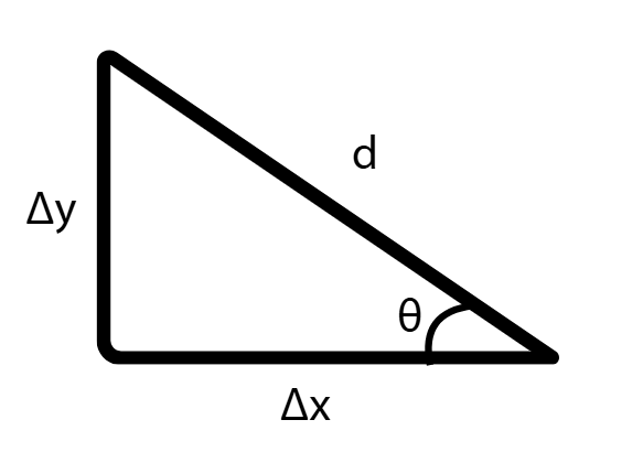
Based on this triangle, we can use trigonometry to calculate our change in x and y position over a timestep using the equations below:

\Delta x = d\cos\left(\theta\right) \\ \Delta y = d\sin\left(\theta\right)

This is a really simple positional tracking method that we can iterate every timestep to constantly track where our robot is. Now we have basic odometry!

Arc Odometry

Generally, robots don’t travel in perfectly straight lines. This is especially the case if more complex motions are being moved, causing the robot to move in curved motion. Because of this, it can be more accurate to approximate robot’s motions each timestep with a circular arc rather than a straight line. To do this, we need a some more complex calculations.

Note: Don’t worry, the calculations are actually fairly simple.

To begin, we must set up a circular arc representing our motions. We will use the variables below:

L - Length of the arc read from an odometry wheel or the drive base (Or both! See the Kalman Filtering page for more information)
d - The distance along a chord that represents the arc, which is the distance from where the robot started to where the robot ended during the timestep
r - The radius of the arc
$\theta_{initial}$ - The heading at the beginning of the timestep
$\theta_{final}$ - The heading at the end of the timestep
$\Delta \theta$ - The change in heading during the timestep

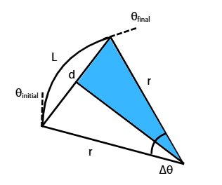
Diagram of the robot's motion as a circular arc

After representing the robot’s motion over a timestep as an arc, it still isn’t apparent how to proceed to get the $\Delta x$ and $\Delta y$ positions of the robot during the timestep. We need a target of something to solve for. That’s where the chord drawn on the figure comes in handy, as if we find the distance between our starting point and end point, we can use basic trigonometry to get our robots change in x and y positions.

To get this distance, we first need to calculate the radius of the arc. We must first convert our theta into radians, as this allows us to use the simple arc length equation, $L = \theta r$ , to calculate the radius. To do this, we must use the following conversion between degrees and radians:

\theta_{radians} = \frac{\pi}{180} \theta_{degrees}

Note: Typically, it isn’t a bad idea to make some constant in your code or an Angle class to make converting between radians and degrees easier. However, using this equation is fine if you don’t know how to do otherwise.

Once we have theta in radians, we can proceed to calculate the radius of our arc (using circular arc length formula):

L = \theta r \\ r = \frac{L}{\theta}

With simple algebra, we have converted the arc length equation into an equation that allows us to calculate the radius of the arc. Now, we are able to move on to calculating the chord distance.

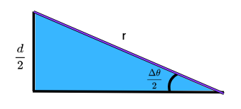
First, we can take part of the other diagram, making a triangle as shown above. Now, we can use very basic trigonometry to calculate our chord length with the equations below:

o=\frac{d}2\\h=r\\\frac{o}{h} = \sin(\frac{\Delta\theta}{2})\\\implies d=2r*\sin(\frac{\Delta\theta}{2})

Now we have the distance of a chord that approximates our robot’s movement! We can then use simple trigonometry to convert that into $\Delta x$ and $\Delta y$ values globally.

We can use this idea again, where the distance is the hypotenuse of a triangle, and given a heading, we can get our global $\Delta x$ and $\Delta y$ values. The only problem is that it isn’t initially clear what value to use for $\theta$ as when moving along an arc, we didn’t travel at a constant heading. There isn’t a nice way to determine what angle the chord is facing based only off of the initial or final heading. However, if we average our initial and final headings, we can get a good approximation of the direction we are facing. Thus, we can use the following to calculate our position:

\theta_{avg} = \theta_{final} - \theta_{initial} \\ \Delta x = d\cos\left(\theta_{avg}\right) \\ \Delta y = d\sin\left(\theta_{avg}\right)

There we go! Now we have fully calculated our change in position by approximating our robot’s motion with an arc. It’s a fairly simple method to obtain more accurate positional tracking than Linear Odometry.

Not an AD: Do you wish that Horizontal Odometry was covered in this tutorial after having figured it out completely? Do you wish that the Odometry explanation was better? Are you just bored and want something to do? Please contribute!